What You Will Learn
- How BM25 keyword retrieval works
- How dense retrieval uses embeddings and vector similarity
- Why hybrid retrieval is used in production RAG systems
- How Reciprocal Rank Fusion (RRF) merges retriever results
- How reranker models improve retrieval accuracy
Effective RAG pipelines require strong retrievers. Otherwise, we may either confuse the LLM with too much information or pass incorrect information to the LLM as context. As we know, building a RAG system involves using context to generate the right response with an LLM, and this context comes from the retriever. Using the context retrieved from the retriever, the LLM generates a response. That is why this pipeline is called a Retrieval Augmented Generation (RAG) pipeline.
In this article, I share practical insights and lessons learned while building Agentic AI solutions and Retrieval-Augmented Generation (RAG) pipelines.
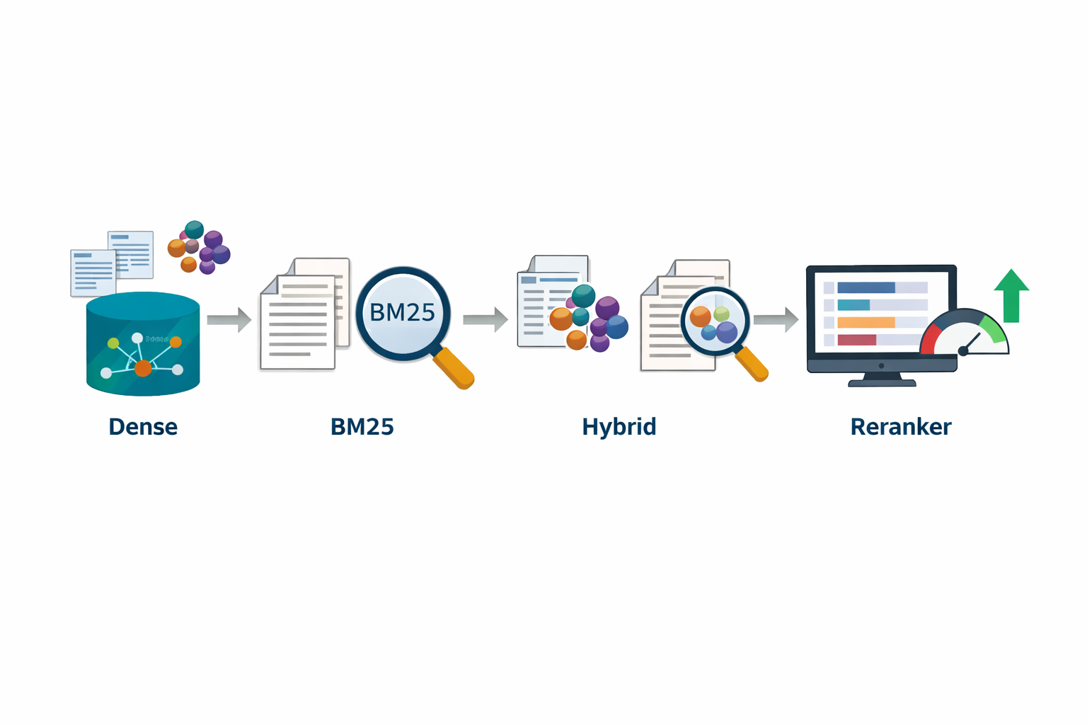
Retrieval is one of the most important parts of the architecture when building RAG solutions. Today, there are several types of retrieval approaches, and some of the most important ones are listed below.
1. Dense Retrieval
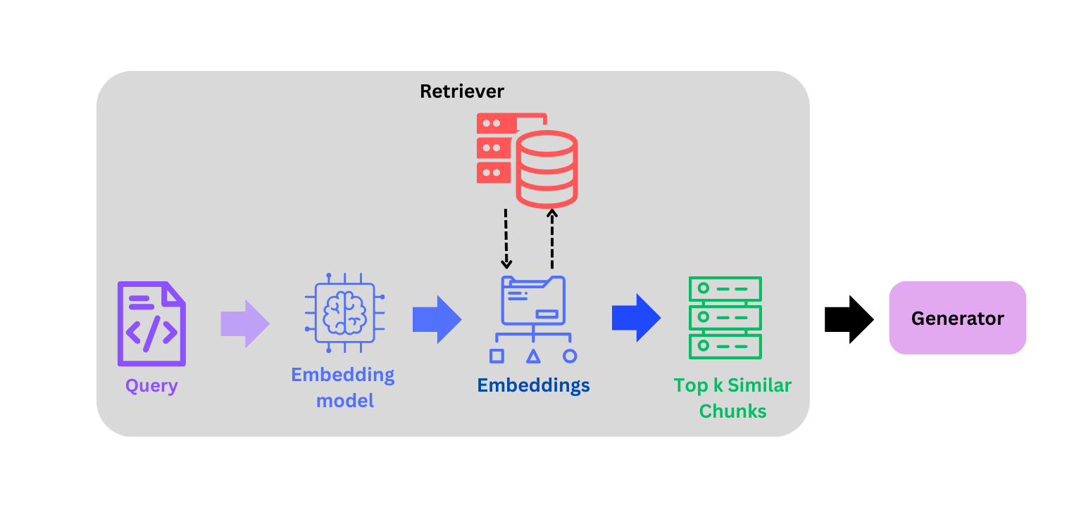
This a well-known similarity search–based retrieval approach where:
- The query is converted into embeddings using an embedding model such as gemini-embedding-001.
- A similarity search is then performed between the query embedding and the embeddings of the entire corpus.
- The top k most similar chunks with respect to the query are returned.
This retrieval method extracts the most relevant chunks for a query by leveraging the semantic relationships captured during the embedding process. embedding process.
Advantages:
- Dense retrieval understands the semantic relationship between words. Even if the query and the document use different wording, the system can still retrieve relevant results because embeddings capture contextual meaning.
- It works well for conversational or complex queries where exact keyword matching may fail, making it highly suitable for modern LLM-based RAG systems.
Disadvantages:
- Computationally expensive
- Dense retrieval sometimes overlooks exact terms such as product names, IDs, codes, or rare keywords, which can lead to missing highly relevant documents.
2. BM25 Retrieval
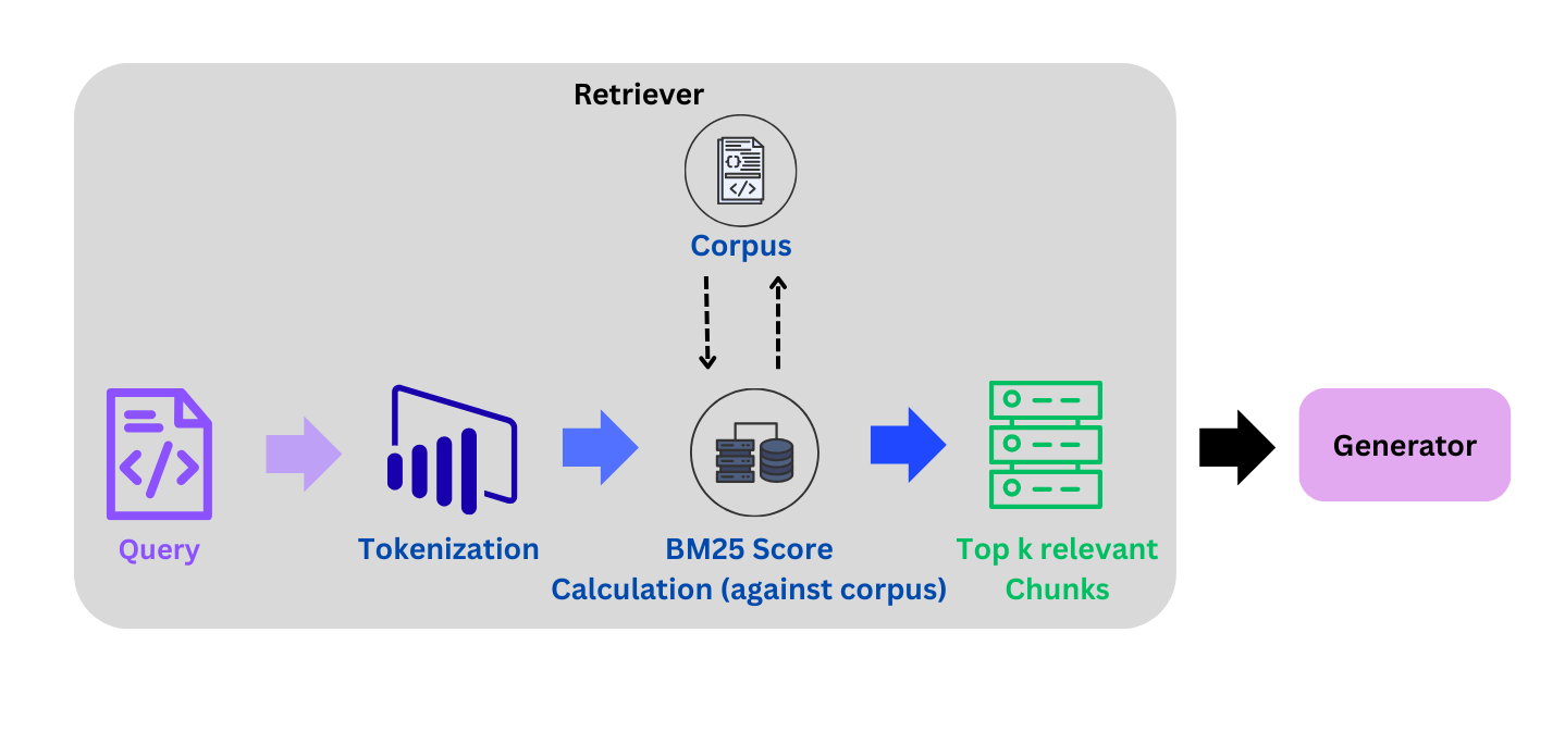
This retrieval approach is known for keyword-based matching. It splits documents (sentences or paragraphs) into words or smaller tokens and uses a frequency-based scoring mechanism to retrieve the most relevant chunks.
For example:
Query = “What is late fee?”
Step 1: Define the corpus, where each chunk will be treated as document
Corpus = [
"Late payment fee is charged when the minimum amount due is not paid.",
"The bank charges a late fee if the payment is delayed.",
"A late fee late fee late fee is applied when you miss the payment deadline.",
"Credit card interest and finance charges apply when balance is unpaid."
]
Notice here:
- document 3 repeats late fee
- document 4 has no relevant terms
Step 2: Split query into tokens:
Tokens = ["What", "is", "late", "fee", "?"]
In most cases we remove stop words and punctuations, so after necessary cleaning tokens become:
Tokens = ["late", "fee"]
Step 3: BM25 scoring (most important step)
BM25 computes a relevance score between the query and each document.
The formula is:
BM25(D, Q) = Σ IDF(qi) * ((f(qi, D) * (k1 + 1)) /
(f(qi, D) + k1 * (1 - b + b * |D| / avgDL)))
| Term | Meaning |
|---|---|
| f(qi, D) | frequency of term in document |
| IDF | inverse document frequency |
| D | Document |
| avgDL | average document length |
| k1 | term frequency scaling parameter |
| b | document length normalization |
It gives values like: [1.5, 0.75, etc.]
Earlier frequency-based scoring techniques such as TF-IDF were commonly used. BM25 improves upon these approaches by penalizing excessive repetitions of words in a document, ensuring that a higher frequency of a term does not automatically result in a higher relevance score.
For example look at document 3:
"A late fee late fee late fee is applied..."
Term frequency:
f("late") = 3
f("fee") = 3
If we used TF-IDF, the score would increase linearly:
score ∝ frequency
Meaning repetition would inflate the score artificially.
BM25 Fixes This
BM25 uses term frequency saturation. Instead of increasing linearly, the score grows slowly.
Example:
| Frequency | TF-IDF | BM25 |
|---|---|---|
| 1 | 1 | 1 |
| 2 | 2 | 1.5 |
| 3 | 3 | 1.7 |
| 10 | 10 | ~2 |
So repeating words does not dominate the ranking. This is where BM25 performs better than TF-IDF.
Step 4:
Calculate the scores for the given query using the above formula. BM25 evaluates each document.
| Document | Score |
|---|---|
| Doc 2 | highest |
| Doc 1 | high |
| Doc 3 | medium |
| Doc 4 | low |
Once we have documents sorted via relevance scores, we choose the top k chunks as context and pass them to the LLM to generate the response.
Advantages:
- Faster and keyword frequency based, so no need of embedding API calls.
- Efficient and computationally inexpensive.
Disadvantages:
- Strong keyword matching BM25 performs very well when the query contains exact keywords present in the documents. It is particularly effective for retrieving documents containing specific terms such as product names, error codes, or domain-specific terminology.
- BM25 does not understand semantic relationships between words, so it may fail when the query uses different wording or synonyms.
Having said that, BM25 is widely used in production search systems such as Elasticsearch, OpenSearch, and Lucene.
3. Hybrid Retrieval
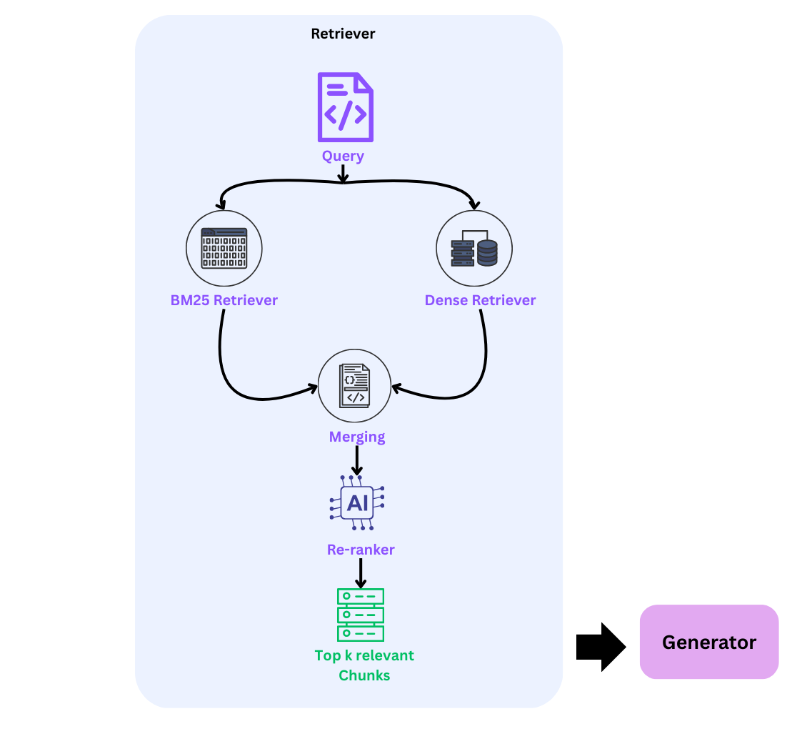
Today, this retrieval approach is used by many systems such as Perplexity AI, Elastic (Elasticsearch), and Amazon OpenSearch. Hybrid search combines the best of both worlds by retrieving chunks based on both semantic relationships (dense retrieval) and lexical relationships (keyword-based retrieval).
Step 1: First, retrieve the top k chunks using dense retrieval.
Step 2: Then, use BM25 retrieval to extract another set of top k chunks.
Step 3: Merge the results from both retrievers using methods such as naive merge (union), score fusion (weighted sum), or the most commonly used method, Reciprocal Rank Fusion (RRF).
RRF Formula:
score = 1 / (k + rank)
Where:
- k = a scaling factor (a constant value, typically 60)
- rank = the position of the document in the retriever’s result list
Step 4:
To make hybrid search stronger, we add an additional layer in the form of a reranker model. This ensures that the retrieval system passes only the most relevant chunks to the LLM instead of sending all retrieved chunks (for example, the top 20), which may introduce noise and confuse the model.
Before moving further, let us briefly understand what a reranker model does.
The objective of a reranker model is to score the query with respect to each of the retrieved chunks. The model assigns a relevance score between 0 and 1 to every chunk. Based on these scores, the chunks are sorted, and only the top k most relevant chunks are selected and passed as context to the LLM.
We use a reranker model to ensure that only the most relevant chunks are passed to the LLM. Without this step, the system may send all chunks combined from the dense and BM25 retrievers, which can include irrelevant information. This noise may confuse the LLM and lead to less accurate responses.
Mostly used reranker models:
| Model | Description |
|---|---|
| cross-encoder/ms-marco-MiniLM-L-6-v2 | fast production reranker |
| cross-encoder/ms-marco-MiniLM-L-12-v2 | better accuracy |
| cross-encoder/ms-marco-electra-base | larger and stronger |
Step 5: Based on the reranker scores, we select the top k most relevant chunks, which then become the context passed to the LLM.
While dense retrieval performs strongly on smaller semantic datasets, hybrid retrieval provides additional robustness as dataset size and lexical diversity increase.
Advantages:
-
Combines semantic and keyword matching
Hybrid retrieval leverages both dense retrieval (semantic understanding) and BM25 (keyword matching). This allows the system to capture conceptual meaning while also ensuring exact keyword matches are not missed. -
More robust across diverse datasets
As datasets grow in size and lexical diversity, hybrid retrieval performs more consistently because it balances semantic similarity with lexical relevance.
Disadvantages:
-
Higher system complexity
Hybrid retrieval requires running multiple retrieval systems (dense and lexical) and then merging the results using techniques such as RRF or score fusion. This increases architectural complexity. -
Higher computational cost and latency
Since two retrieval processes are executed and often followed by a reranking step, hybrid retrieval can increase compute requirements and response latency compared to single-retriever systems.
Implementation
Objective: Create a retrieval system for credit card documentation to answer the most frequently asked questions from customers.
Dense Retrieval: Dense retrieval evaluation scores
| Metric | Score |
|---|---|
| Precision@5 | 0.304 |
| Recall@5 | 0.895 |
| MRR | 0.914 |
If you want to build this pipeline from scratch using an effective chunking strategy, you can read this baseline retriever for RAG systems.
BM25: Lexical retrieval pipeline
| Metric | Score |
|---|---|
| Precision@5 | 0.226 |
| Recall@5 | 0.671 |
| MRR | 0.663 |
Here, we can observe that the scores for this document are lower compared to dense retrieval.
Hybrid Retrieval
| Metric | Score |
|---|---|
| Precision@5 | 0.292 |
| Recall@5 | 0.871 |
| MRR | 0.838 |
Here, we can see that dense retrieval performs marginally better than hybrid retrieval for this case because the dataset is relatively small. Hybrid retrieval typically performs better on larger datasets, which is why many systems such as Elasticsearch and Perplexity use this approach.
When to Use What
| Retrieval Type | Use Cases | Reason |
|---|---|---|
| Dense Retrieval | semantic search, natural language queries, small datasets, paraphrased queries | Embeddings capture semantic similarity between query and documents |
| BM25 | keyword search, product names, error codes, IDs, exact term matching | Strong lexical matching using term frequency scoring |
| Hybrid Retrieval | large datasets, enterprise knowledge bases, mixed query patterns, production RAG systems | Combines semantic and keyword retrieval for higher robustness |
Conclusion
Depending on the problem statement, we need to design the retrieval pipeline in such a way that the system consistently passes the most relevant chunks to the LLM. This helps the model generate accurate responses. In general, hybrid retrieval tends to perform better on larger datasets and improves the overall accuracy of retrieval.
Until next time, Happy learning!
Full code repo: View on GitHub
LinkedIn profile: Connect on LinkedIn
← Back to Articles