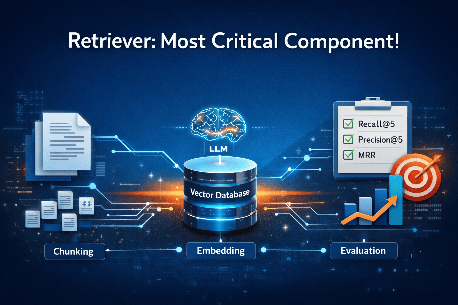
Today, many engineers are building Retrieval-Augmented Generation (RAG) systems. One of the most important components of a RAG system is the retriever. If the retriever is not accurate, the system suffers from the classic problem of "garbage in, garbage out."
If the retriever provides irrelevant or incorrect context, the language model may generate inaccurate responses. Therefore, building a reliable and accurate retriever is important for the overall performance of a RAG system.
In this article, we will build a baseline retriever and evaluate its performance. In the upcoming articles, we will progressively improve this system and move toward building a production-grade retriever that returns the most relevant and accurate chunks for a given query.
The retriever
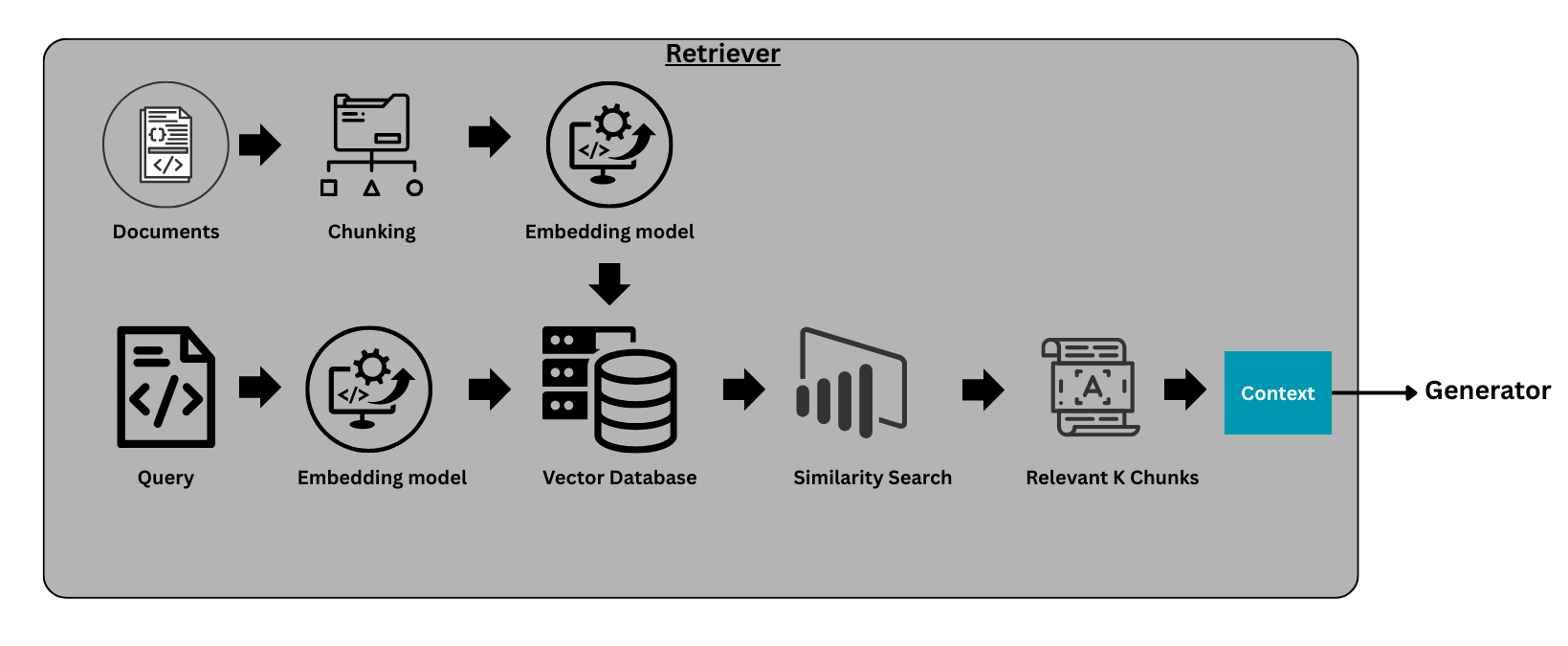
As discussed earlier, retriever is the most important component of a RAG system. It fetches the relevant information from the knowledge base, which becomes the context for the model as shown in the above diagram. Using this context, along with the set of instructions provided through the prompt, the LLM generates a response to the query.
The reason we need external context is that large language models (LLMs) are powerful, but their knowledge is static and limited to the data available during training. If you ask questions about recent events, new regulations, or company-specific information, the model may fail to provide accurate answers.
To solve this problem, we build a knowledge base containing relevant information, which the generator later uses as context to generate responses. Next, we will walk through the key components required to build a baseline retriever.
Chunking (A Critical Component of the Retriever)
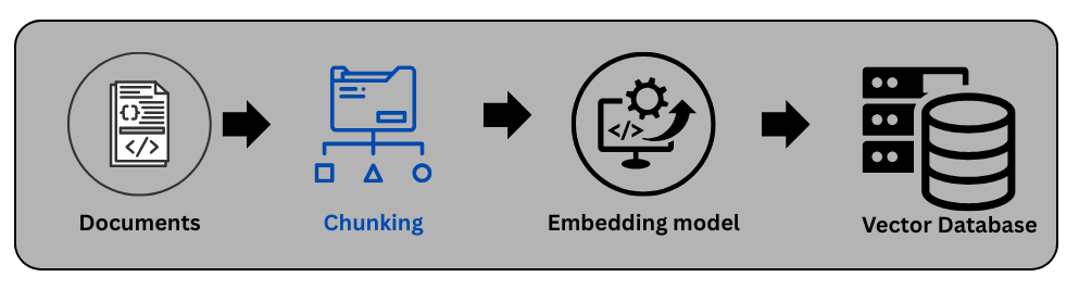
Chunking is a simple yet critical component of a retriever. It refers to the process of splitting a long document into smaller chunks in a strategic way so that, when a query is passed to the system, the retriever can return the most relevant pieces of information.
We perform chunking because storing an entire long document directly in a vector database is not effective for retrieval. Instead, the document is divided into smaller chunks, each chunk is converted into an embedding, and these embeddings are stored in a vector database such as FAISS.
Chunks are the pieces of information that the generator uses to produce a response. If chunking is not done properly, similarity search may fail to retrieve the most accurate and relevant chunks.
For example, if the chunk size is too large, similarity search may not work effectively because the chunk may contain too much unrelated information. On the other hand, if the chunk size is too small, we may lose important context and miss relevant information.
Therefore, choosing an appropriate chunking strategy is very important for the retriever. There are several chunking techniques that can be used depending on the type of documents and the use case. In the following sections, we discuss several commonly used chunking techniques.
1. Fixed-Size Chunking:
In this approach, documents are split into chunks containing a fixed number of tokens or characters (e.g., 300–500 tokens). For example, Chunk 1 may contain tokens from 0 to 400, Chunk 2 from 401 to 800, and so on.
Advantages:
- Simple and fast to implement.
Disadvantages:
- It may break semantic boundaries. For example, half of a sentence may appear in Chunk 1 while the remaining half appears in Chunk 2.
2. Overlapping Sliding Window Chunking:
This technique is similar to fixed-size chunking, with one key difference: each chunk overlaps slightly with the previous chunk to preserve context. For example, Chunk 1 may contain tokens from 0 to 400, while Chunk 2 may contain tokens from 350 to 800. In this case, there is a 50-token overlap between the chunks to maintain contextual continuity.
Advantages:
- Easy to implement.
- Works well for most types of documents
Disadvantages:
- Requires storing more embeddings compared to fixed-size chunking.
3. Semantic Chunking
In this approach, documents are first broken down into sentences or groups of sentences. These sentences are then converted into embeddings, and semantically similar sentences are grouped together. Each group of related sentences forms a chunk. For example, Chunk 1 may include the first 10 sentences that discuss the same topic.
Advantages:
- Preserves semantic meaning..
- Works well for most types of documents
Disadvantages:
- For large documents, it can become computationally expensive due to the need to generate embeddings and cluster similar sentences.
4. Structure-Based Chunking (Section / Heading Based)
In this type of chunking, we examine whether the document has a clear structure, such as sections and subsections. If the document is well structured, these sections can be used as natural chunk boundaries. For example, the definitions section may be divided into Chunk 1 to Chunk 3 or the fees section may be divided into Chunk 4 to Chunk 6, and so on.
Advantages:
- Maintains logical context.
- Works very well with structured documents such as legal agreements, policies, and terms and conditions.
Disadvantages:
- Can produce uneven chunk sizes. To address this, a hybrid approach combining structure-based chunking with fixed-size or overlapping chunking can be used.
5. Hierarchical Chunking
In hierarchical chunking, documents are split into multiple levels of chunks.
Example structure:
    Document
    │
    ├── Section (Parent)
    │   ├── Paragraph (Child)
    │   ├── Paragraph (Child)
    │
    ├── Section
During retrieval, the system first retrieves child chunks (smaller units of text) and then returns the parent section to the LLM to provide broader context.
Advantages:
- Improves retrieval precision.
Disadvantages:
- Requires a more complex architecture.
- Higher storage requirements due to the need to maintain parent–child relationships.
Retriever Implementation
Objective: We will create a retriever using credit card terms and conditions document. Let’s assume this retriever is getting used in RAG system to answer any customer questions related to credit cards.
Document description: Here input document is credit card terms and conditions, it includes all the charges related information like late fees, annual fees, etc. It also includes all the basic details of interest calculations etc.
Let’s determine which chunking technique is most appropriate for our use case. If we look at the document we are working with, it is well-structured and organized into clear sections. For example, the document contains sections such as Definitions, Fees, Credit Limit, Use of Card, and Billing & Settlement, each describing a specific aspect of the credit card agreement.
There are several reasons why section-based chunking works well for this document:
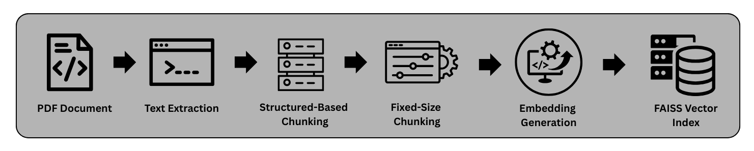
The document already contains clearly defined headings and sections, making it easier to split the content logically. Instead of splitting the document arbitrarily by token size, we treat each section as a logical chunk. This helps preserve the semantic meaning and context of the information within that section. To avoid the problem of uneven chunk sizes, we use a hybrid approach. This means we will use both Structure-Based Chunking (Section-wise) and Fixed-Size Chunking (400-word limit).
Step 1:
We use a PDF reader to load the document and regular expressions to detect sections such as Definitions, Fees, and Credit Limit. The following helper function extracts all sections from the document.
    def split_sections(text):

        sections = []
        current_section = None
        expected_section = 1

        lines = text.split("\n")

        for line in lines:

            line = line.strip()
            if not line:
                continue

            match = re.match(r'^(\d{1,2})\.?\s+(.+)', line)

            if match:

                section_number = int(match.group(1))

                if section_number == expected_section:

                    if current_section:
                        sections.append(current_section)

                    current_section = {
                        "header": f"{section_number}. {match.group(2)}",
                        "content": line + "\n"
                    }

                    expected_section += 1
                    continue

            if current_section:
                current_section["content"] += line + "\n"

        if current_section:
            sections.append(current_section)

        return sections
Step 2:
Now we will apply fixed-size chunking to avoid the problem of uneven token distribution. In this case, we use a chunk size of 400 tokens, as shown in the code below. However, in the metadata we preserve the section name for each chunk.
        def chunk_sections(sections, chunk_size=400):

            chunks = []
            chunk_id = 0

            for sec in sections:

                words = sec["content"].split()

                for i in range(0, len(words), chunk_size):

                    chunk_text = " ".join(words[i:i+chunk_size])

                    chunks.append({
                        "chunk_id": chunk_id,
                        "section_title": sec["header"],
                        "text": chunk_text,
                        "source": "axis_credit_card_doc"
                    })

                    chunk_id += 1

            return chunks
This helps maintain consistent chunk sizes and improves retrieval quality.
Now that we are done with chunking, the next step is to generate embeddings so that similar chunks have similar vector representations. For embedding generation, we use Gemini’s embedding model (gemini-embedding-001). This model takes text as input and returns vectors of shape (n, 3072).
        result = client.models.embed_content(
            model="gemini-embedding-001",
            contents=texts,
            config=types.EmbedContentConfig(task_type="SEMANTIC_SIMILARITY")
        )
Note: This model is available through the paid Gemini API. You can also use open-source embedding models such as intfloat/e5-large-v2 from Hugging Face.
Step 3:
As the next step, we store these embeddings in a vector database. For this example, we use FAISS (Facebook AI Similarity Search ), an open-source library developed by Meta for efficient similarity search.
We store the FAISS index object locally and use it later to retrieve relevant information. In addition, we store the document chunks along with their metadata, which will be used at query time to fetch the corresponding text for the retrieved embeddings.
        embeddings = np.array(
            [chunk["embedding"] for chunk in embedded_chunks]
        ).astype("float32")

        dimension = embeddings.shape[1]

        index = faiss.IndexFlatL2(dimension)

        index.add(embeddings)

        faiss.write_index(index, "axis_card_faiss.index")
Step 4:
Now we are ready with our knowledge base, which is stored in a vector database. We will create a helper function that accepts a customer message or question and retrieves the most relevant chunks from the vector database. These retrieved chunks will serve as context for the LLM, which will use this information to generate a response.
    def similarity_search(query_vector, top_k=3):

        query_vector = np.expand_dims(query_vector, axis=0)

        distances, indices = index.search(query_vector, top_k)

        results = []

        for idx in indices[0]:

            chunk = chunks[idx]

            results.append({
                "chunk_id": chunk["chunk_id"],
                "section_title": chunk["section_title"],
                "text": chunk["text"]
            })

        return distances, indices,results
Retriever Evaluation (Critical step in the architecture)
Now that our retriever is ready, the next step is to perform one of the most important parts of the process: evaluating the retrieval system. We do this to verify whether the system is returning the correct context for a given query. To measure the performance of our retriever, we will use the following evaluation metrics.
For these metrics, we will rely on a ground truth dataset, as shown below. The idea is to manually create this ground truth by examining the chunks generated during the chunking step and identifying which chunks are relevant for a given query. In other words, we are creating labeled data that allows us to measure the accuracy of our retriever.
For the purposes of this article, we use a relatively small ground truth dataset. However, in real-world systems, evaluation is typically performed using a much larger set of labeled queries.
1. Recall@5
This metric measures how many of the relevant chunks were successfully retrieved in the top 5 results.
Formula:
Recall@K = relevant retrieved / total relevant
Example:
Expected relevant chunks:
[7, 14, 0]
Total relevant chunks = 3
Retrieved chunks:
[14, 2, 7, 30, 1]
Relevant retrieved chunks:
[14, 7]
Total relevant retrieved = 2
Recall@5 = 2 / 3 = 0.67
Interpretation:
A high recall score means the retriever is not missing important information.
2. Precision@5
This metric measures how many of the top 5 retrieved chunks are actually relevant.
Formula:
Precision@K = relevant retrieved / K
Example:
In our case:
K = 5
Retrieved chunks:
[14, 2, 7, 30, 1]
Relevant retrieved chunks:
[14, 7]
Total relevant retrieved = 2
Precision@5 = 2 / 5 = 0.4
Interpretation:
A high precision score means the retriever is returning mostly relevant results with minimal noise.
3. MRR (Mean Reciprocal Rank)
This metric measures how early the first relevant result appears in the ranking. LLMs perform better when the most relevant context appears earlier in the retrieved results.
Formula:
Reciprocal Rank = 1 / rank of first relevant result
Example 1:
Retrieved:
[14, 2, 7, 30, 1]
Relevant chunks:
[14, 7]
The first relevant chunk (14) appears at Rank = 1
RR = 1 / 1 = 1.0
Example 2:
Retrieved:
[2, 5, 14, 7, 30]
Relevant chunks:
[14, 7]
The first relevant chunk (14) appears at Rank = 3
RR = 1 / 3 = 0.33
Mean Reciprocal Rank (MRR)
MRR is calculated by averaging the reciprocal ranks across multiple queries.
MRR = (1.0 + 0.33) / 2 = 0.665
Interpretation:
A higher MRR indicates that relevant results tend to appear earlier in the ranking.
These metrics help evaluate the effectiveness of the retriever in a RAG system. In real-world production systems, additional techniques are often applied to further improve retrieval quality, as discussed below.
| Metric | Focus | Business Priority |
|---|---|---|
| Precision@K | Correctness of retrieved chunks | Reduce noise |
| Recall@K | Coverage of relevant information | Avoid missing context |
| MRR | Ranking quality | Best answer appears early |
Helper function used to calculate accuracy of our retriever system:
    precision_scores = []
    recall_scores = []
    mrr_scores = []

    K = 5

    for item in result_eval:

        retrieved = item["indices"][0].tolist()
        relevant = item["expected_chunk"]

        # Count how many retrieved are relevant
        relevant_retrieved = len(set(retrieved) & set(relevant))

        # Precision@K
        precision = relevant_retrieved / K
        precision_scores.append(precision)

        # Recall@K
        recall = relevant_retrieved / len(relevant)
        recall_scores.append(recall)

        # MRR (first relevant chunk rank)
        rank = None
        for i, r in enumerate(retrieved):
            if r in relevant:
                rank = i + 1
                break

        if rank:
            mrr_scores.append(1 / rank)
        else:
            mrr_scores.append(0)

    precision = np.mean(precision_scores)
    recall = np.mean(recall_scores)
    mrr = np.mean(mrr_scores)

    print("Precision@5:", precision)
    print("Recall@5:", recall)
    print("MRR:", mrr)
This step is extremely crucial in a retriever system. If we want to avoid incorrect responses or, as discussed earlier, the “garbage in, garbage out” problem, this stage becomes very important.
What we have built so far can be considered a baseline retriever. While it may perform well on a small sample dataset, its performance on larger datasets is uncertain. To further improve the accuracy of a retriever, several techniques are commonly used:
- 1. Hybrid Search: combining BM25 (keyword search) with vector similarity search for better retrieval.
- 2. Reranking Models: models that assign relevance scores to retrieved chunks based on their semantic similarity to the query.
- 3. Query Expansion: expanding the user query with related terms to improve recall and retrieval quality.
In the next article, we will enhance our baseline retriever by integrating hybrid search and evaluating the system on a larger dataset.
Until then, happy learning!
Resources:
- GitHub Repository: View the complete code
- LinkedIn Profile: Connect with me on LinkedIn